Using the GUI

CloudScope provides a desktop and browser GUI for loading raw image files, visualizing image data, selecting ROIs, and running supported analysis workflows. Current quantitative analysis workflows are designed for line scan kymographs.

CloudScope is designed around a simple workflow: load data, visualize what you need, define or select ROIs, run analysis, and review or export results.

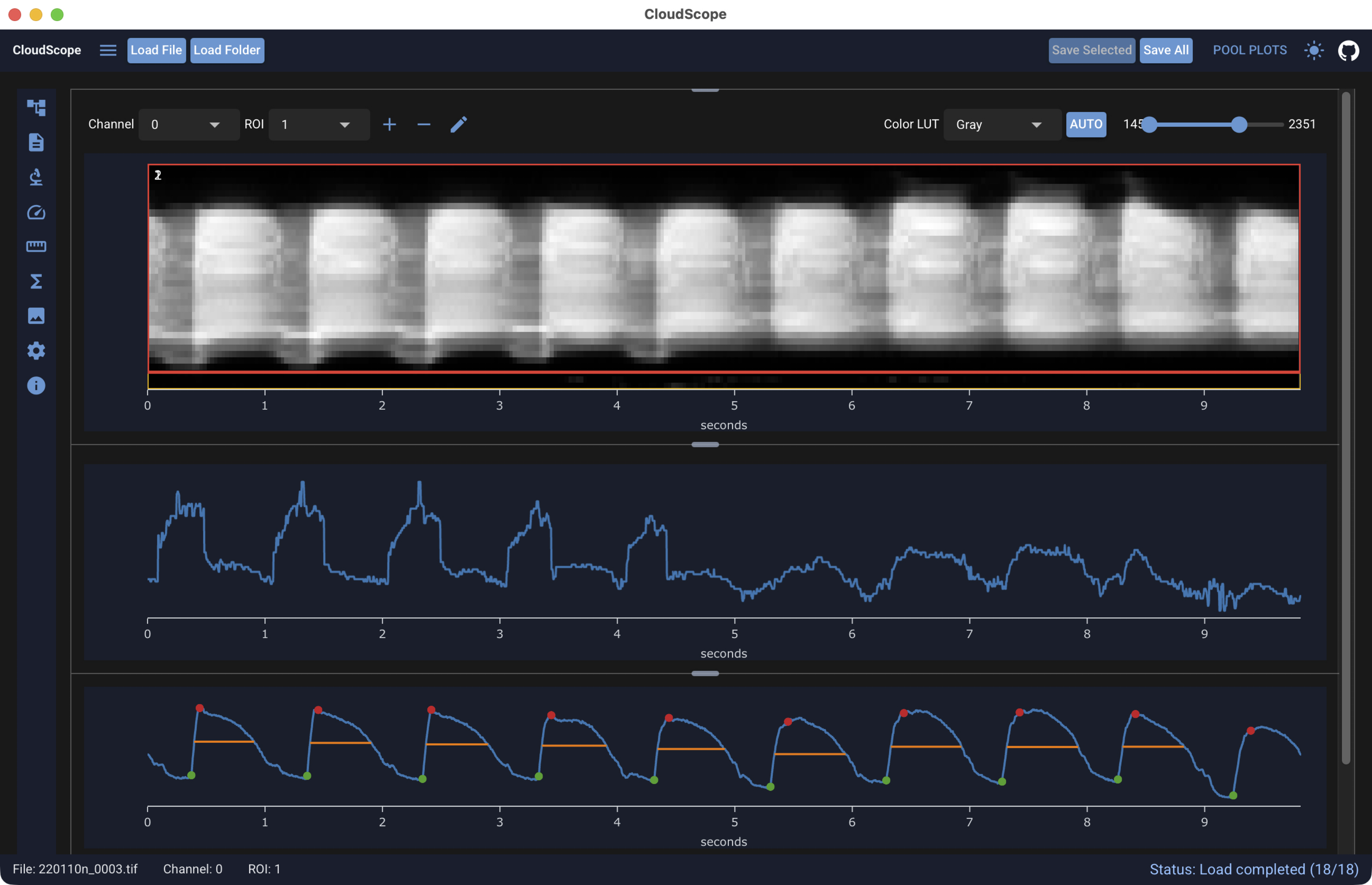
Main areas shown above:

• Left toolbar — icon column that opens side panels (file list, metadata, analyses, and settings).
• Loading and saving — CloudScope title, history menu (), load and save buttons, and theme controls.
• File list — tree of loaded files at the top of the main workspace (full column set). The left-toolbar File List panel shows the same data in a compact layout.
• Image viewer — kymograph display with ROI overlays; the image toolbar sits above it.
• Analysis plot — velocity or diameter trace for the current selection.
• Peak detection plot — df/f0, derivative, and peak markers when peak detection applies.
• Pool plots — optional right-side panel (Pool plots) for folder-wide velocity and peak comparisons; open with Pool Plots near the top of the window.

Getting started with sample data

The fastest way to explore CloudScope is to load example data from the cloudscope-data repository. Open the history menu () next to the load buttons and choose:

Menu item	Sample content
Load Velocity Sample Data	OIR kymograph data for velocity analysis demos
Load Diameter Sample Data	TIFF kymograph data for diameter analysis demos

CloudScope downloads the archive on first use, verifies it, and caches it locally. The loaded folder appears in the file list like any other folder load.

Sample data is the recommended first step when trying the application, confirming a fresh installation, or working through the recipes.

Basic workflow

A typical CloudScope session is:

1. Open CloudScope in the browser or launch the desktop app.
2. Load sample data from the history menu, or open local image files.
3. Select an image file in the file list.
4. Visualize the image and choose or create an ROI.
5. Run a supported analysis.
6. Review results in the GUI.
7. Save or export results.

For comparing analysis results across a loaded folder, see Pool plots.

Supported file formats

CloudScope loads the same formats in the desktop app and the browser app. Discovery and loading are provided by AcqStore — see Loading an image for loader detail.

Commercial microscopy formats

Format	Extension	Notes
Olympus / Evident	.oir	May include a reference/overview image. Physical units and reference spatial scales are loaded when available.
Zeiss	.czi	May include a reference/overview image and scan path. Physical units are loaded when available.
Nikon	.nd2	Nikon NIS-Elements acquisitions.

Open image formats

Format	Extension	Notes
TIFF	.tif	Generic TIFF, including multi-channel images.
OME-Zarr	.ome.zarr	Directory-backed OME-Zarr stores (load).

Notes

• Physical units. OIR and CZI often populate Y/X unit size and labels. Plain TIFF may lack embedded scaling — use Image header to set or override units, then save.
• Reference images. OIR and CZI often include a reference/overview image and scan-path metadata. See the AcqStore kymograph reference images notebook and Save Reference As Tif in Saved file formats.
• Load reporting. Unreadable files are reported as warnings (missing file, unsupported type, or read error) rather than failing the whole folder load.

CloudScope's CZI and OIR support builds on file-format work by Christoph Gohlke.

Loading and saving

Controls for opening and saving data sit near the top of the window: the CloudScope title on the left, load and save buttons in the center, and theme controls on the right.

Behavior differs slightly between the desktop app and the browser app:

Desktop appWeb app

• Load File — open one supported image file from your computer (native file picker).
• Load Folder — open a folder and load supported image files within it (native file picker).
• Upload File is not shown; the desktop app reads files directly from disk.

• Load File and Load Folder are disabled. Browsers cannot open arbitrary local paths the way the desktop app can. Hover the disabled buttons to see: Local file picker is available in the desktop app.
• Upload File — upload one supported image file from your computer. You can also drop a file onto the upload control.

History menu ()

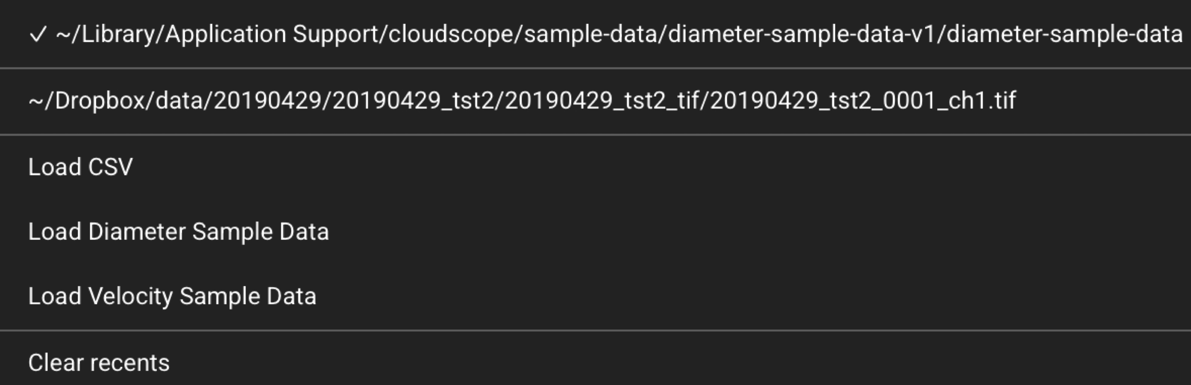
Click the history menu button () to the left of the load buttons. Menu contents appear in this order:

1. Recent folders — one entry per recently opened folder. A check mark (✓) marks the path that matches the current session's last loaded folder. Click an entry to reload that folder.
2. Recent files — one entry per recently opened file (including CSV paths opened as files). A check mark marks the current last-loaded file when applicable.
3. Load CSV — open a CSV file from disk (desktop) or from upload context (web). Used when working with tabular outputs outside the normal image load flow, and to load a randomized file manifest that samples a subset of a large dataset. See the AcqStore randomized file subset notebook and Blinded analysis mode.
4. Load Diameter Sample Data — download and open the diameter-analysis sample dataset from cloudscope-data.
5. Load Velocity Sample Data — download and open the velocity-analysis sample dataset from cloudscope-data.
6. Clear recents — remove all entries from the recent folders and recent files lists (shown when at least one recent path exists).

Saving

On the right side of the load and save row:

• Save Selected — save the currently selected file when it has unsaved changes. Disabled when no file is selected or the selection has no pending changes.
• Save All — save every loaded file that has unsaved changes. Always available when files are loaded.

Saved files include a JSON state file and analysis CSV files next to each source image. See Saved file formats for a full description of what is written for metadata, ROIs, and each analysis type.

Left toolbar

The left toolbar is a column of icons along the left edge of the window. Each icon opens a panel. Click an icon to open its panel; click the same icon again to close the panel and return to the icon-only toolbar.

Tooltip	What it does
File List	Compact tree of loaded files, channels, ROIs, and analyses. See File list below.
Experimental Metadata	Edit experiment metadata fields for the selected file. See Experiment metadata.
Image Header	View header fields from the file format and set physical units and axis labels. See Image header.
Velocity	Configure and run in vivo blood-flow velocity analysis. See Analysis panels.
Diameter	Configure and run vessel diameter analysis. See Analysis panels.
Peak Detect	Configure and run peak detection (for example GCaMP reporter fluorescence). See Analysis panels.
Reference Image	View the reference or overview image and related metadata when the file format provides one (for example Olympus .oir or Zeiss .czi line scan kymographs). When available, this panel can also show the scan path for the line scan. Use Save Reference As Tif to export the reference image (see Saved file formats).
Config	Application settings (text size, folder load depth, table font, auto-contrast percentiles, and blinded analysis mode). See App config and Blinded analysis mode.
App info	Version and build metadata (when available from a packaged or deployed build), log preview, and Open Logs for troubleshooting.

File list

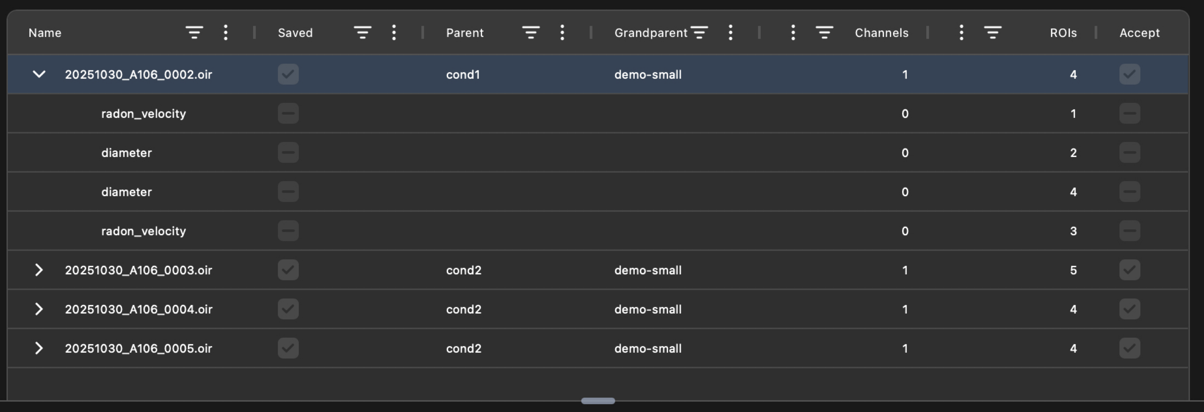
The File list at the top of the main workspace shows loaded files in a tree with the default column set. Open File List on the left toolbar for the same data in a compact panel (fewer columns visible by default; additional columns are available from the context menu).

Selecting a file, channel, ROI, or analysis updates the image viewer, analysis panels, and result plots so they stay in sync with the current selection.

Typical use:

1. Load one or more files.
2. Select the file or channel you want to visualize.
3. Select an ROI or analysis result when available.
4. Use the analysis panels to run or update measurements.

File list context menu

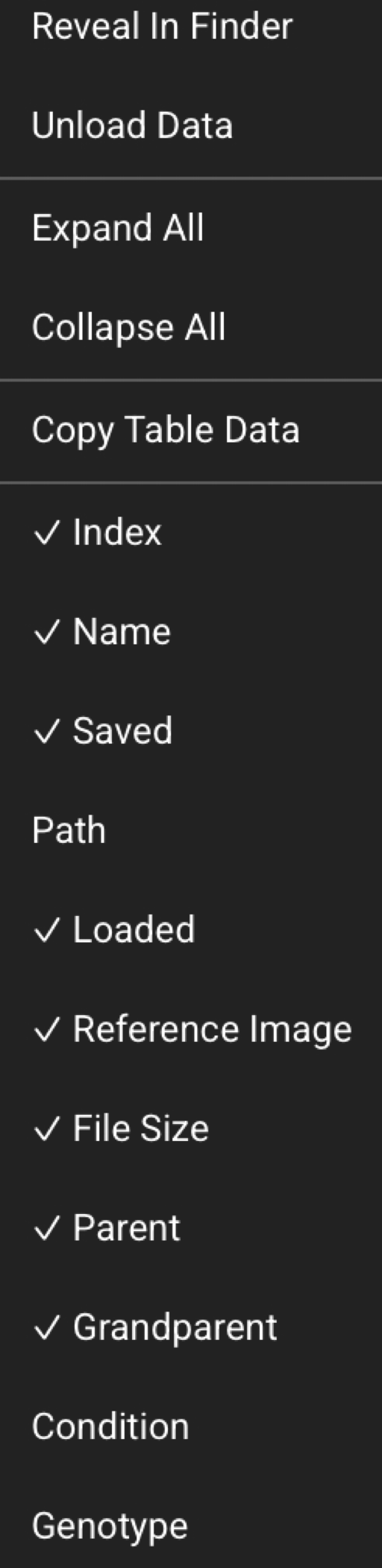
Right-click the file list to open the context menu:

• Reveal In Finder — open the selected file's folder in the system file manager (the menu label follows macOS wording in the app today).
• Save As Tif... — export the selected image as a TIFF file (native save dialog on desktop; browser download in the web app). This writes a new file; it does not replace the source. See Saved file formats.
• Unload Data — free image pixels and analysis data for the selected file while keeping the file entry in the list (useful for large folders).
• Expand All / Collapse All — expand or collapse all tree nodes.
• Copy Table Data — copy the visible tree rows to the clipboard.
• Column toggles (for example ✓ Name, Loaded, Saved, Dims) — show or hide file-list columns. Extra columns remain available from this menu.

Image viewer

The image viewer shows the selected file, channel, and ROI overlays.

Display uses image pyramids so the viewer can show only the resolution needed for the current zoom level — this keeps panning and zooming responsive on large images. Analysis still uses full-resolution source data. Image pixels and analysis results load when you select a file (and can be freed with Unload Data in the file list), so you can browse folders with many hundreds of files without keeping everything in memory at once.

Image toolbar

The image toolbar sits above the image viewer.

Channel and ROI

• Channel — select the active image channel.
• ROI — select the active region of interest.
• Add (+) — add a new ROI.
• Delete (−) — delete the selected ROI.
• Edit — enter ROI edit mode in the image viewer.
• Full width / Full height — resize the ROI to span the full image width or height.
• OK / Cancel — submit or cancel an ROI edit.

Contrast

• Color LUT — colormap for the image display.
• Auto — set display contrast from percentile clipping on the current plane (uses the auto-contrast percentiles in App config).
• Min/max range slider — manual display window; numeric labels show the current min and max values at each end of the slider.

Use this toolbar to adjust what is visible without changing the underlying image data or analysis results.

Image context menu

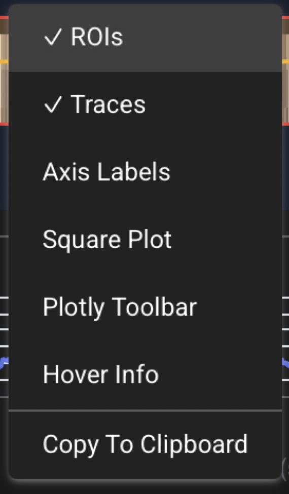
Right-click the image viewer to open the context menu:

• ROIs — show or hide ROI rectangle overlays on the image.
• ROI Labels — show or hide ROI labels (disabled while ROIs are hidden).
• Traces — show or hide analysis trace overlays on the image.
• X Axis Labels / Y Axis Labels — show or hide axis tick labels.
• Square Plot — toggle a square aspect ratio for the plot area.
• Plotly Toolbar — show or hide the zoom/pan toolbar on the plot.
• Hover Info — show or hide hover tooltips on the plot.
• Copy To Clipboard — copy the displayed plot image to the clipboard.

These controls affect how the image is displayed. They do not change the original data.

Analysis panels

Open an analysis from the left toolbar. Step-by-step workflows, screenshots, and saved-file details live on the dedicated recipe pages:

Left toolbar	Recipe
Velocity	In vivo velocity analysis — Radon-transform blood-flow velocity; velocity event analysis is in the same panel
Diameter	Diameter analysis — vessel diameter from line scan kymographs
Peak Detect	Peak detection — functional fluorescence reporters (like GCaMP)

Derived analyses that require velocity results first:

• Velocity event analysis
• Heart rate analysis (notebook today)

Pool plots

After you have analyzed files in a folder, click Pool Plots near the top of the window to open the right-side pool plots panel. Pool plots aggregate in vivo velocity and peak-detection results across the entire loaded folder and refresh automatically when you load files, run analyses, or edit metadata or ROIs.

See Pool plots for an overview, export actions, and example plots. Detailed control documentation is coming soon.